SeQuery provides two navigation interfaces for exploring the GPCR network, as illustrated in Figure 1. We recommend users to use the Chrome browser for better viewing quality. At its homepage (http://cluster.phy.ntnu.edu.tw), users can select the GPCR2841 dataset and explore the GPCR network from the top down (I). Alternatively, users can also submit a query sequence and explore its role in the GPCR network from the bottom up (II).

Fig. 1 Flowchart of the two navigation interfaces of the SeQuery database, including the top-down navigation scheme (I) and the bottom-up navigation scheme (II).
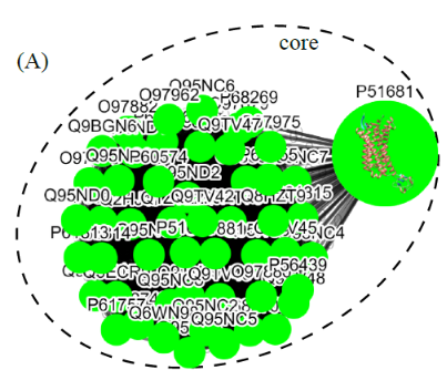
(I) In the top-down navigation scheme, SeQuery first displays the minimum spanning tree (MST) graph of the GPCR superfamily at the third level of clustering, which contains seven GPCR classes as shown in Figure 2. Each node in the network graph represents a GPCR family. The same scheme of colors and shapes as shown in the legend is used to denote the functions of GPCR clusters for all levels of clustering. When users click on a node, as shown in Figure 3, SeQuery shows the MST graph of the superfamily at the 2nd level clustering, centering at constituent clusters of the selected GPCR family. At this second level of clustering, the GPCR superfamily is represented by a MST graph of receptor clusters predicted from the first-level MSC clustering and each node in the graph represents a first-level MSC cluster. Users can explore the 2nd level graph of the network by dragging and zooming the network or locate any GPCR family of interest by clicking on the node in the legend at the left-hand side (SeQuery will center the second level graph at the clusters of the selected family). By clicking on a node in the 2nd level graph, SeQuery shows constituent sequences of the selected cluster in a 1st level graph, as shown in Figure 4 for a Peptide Receptor cluster Pe001 (A) and a Olfactory Receptor cluster Ol001 (B). Each node in a 1st level graph is a GPCR sequence, whose detailed information can be viewed in an information box by clicking on the node. At the first level of clustering, receptor clusters are represented by a tree graph which may or may not contain a core of zero-distance sequences. If a sequence has a known protein structure, such as P51681 in Figure 4(A), its structure will be displayed on the node. When the user clicks on a sequence node, SeQuery displays its sequence and function information, as shown in Figure 5.
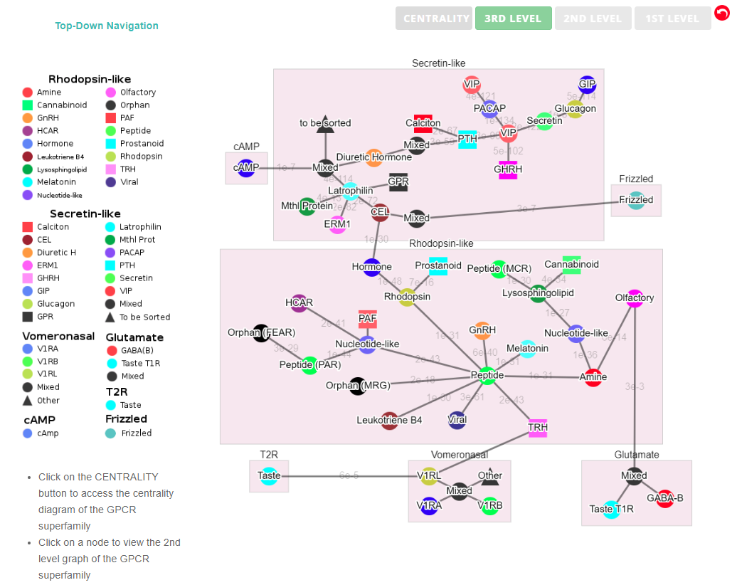
Fig. 2 The third-level minimum spanning tree diagram of the GPCR network with the base dataset. Each node represents a GPCR family. The legend shows the scheme of nodes’ colors and shapes that are used to distinguish GPCR functions annotated in GPCRdb (also labeled on the nodes).
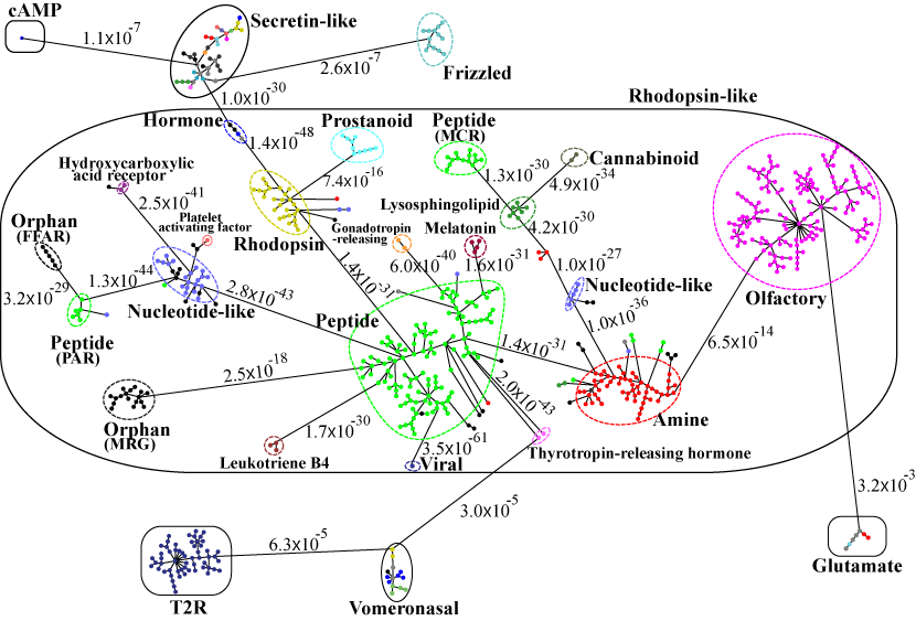
Fig. 3 The second-level minimum spanning tree diagram of the GPCR network in the dataset GPCR2841 (outliers not shown). Here each circle represents an MSC cluster the color of which is according to the function of its constituents. The length of the edges is not proportional to their distance, but the distances between subfamilies and classes are labeled to see their sequence similarity.
 |
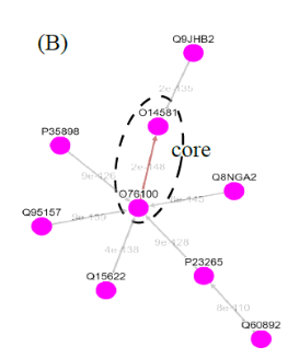 |
Fig. 4 The tree diagrams of first-level GPCR clusters, showing member sequences of cluster Pe001 which has a conservative core (A), and member sequences of cluster Ol001 which has no conservative core (B). In (A) the three-dimensional protein structure of P51681 is displayed in its node.
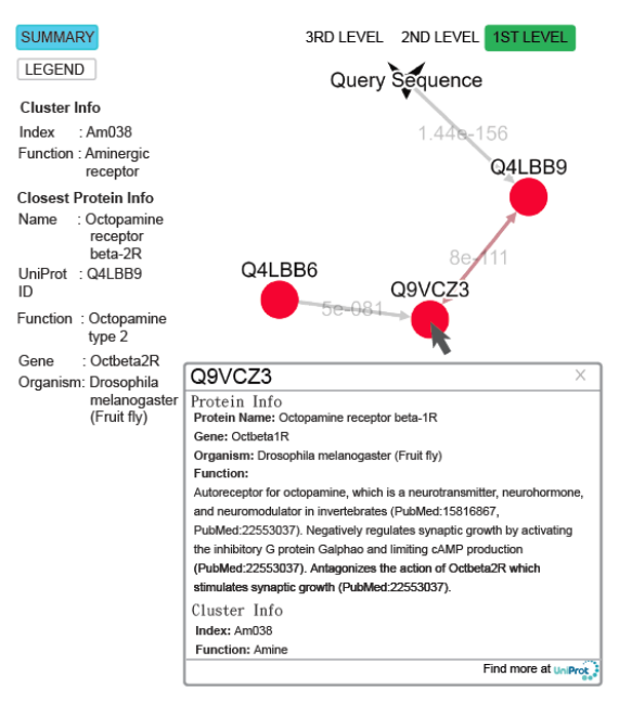
Fig. 5 The query result of the submitted sequence of G3M4F8 in SeQuery, showing the cluster graph at the first level. Both cluster information and closest protein information are shown on the left hand side. Upon clicking on the node Q9VCZ3, a modal box shows both protein information and cluster information of the node.
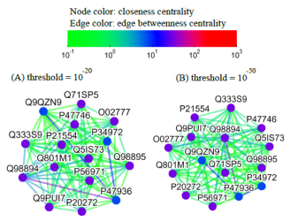
Alternatively, users can select the centrality tab to see the centrality network on the 3rd level graph. When users click a node on the 3rd level network, SeQuery displays various thresholded network graphs showing statistical properties of the corresponding receptor family, as shown in Figure 6 for the Cannabinoid Receptor family in the Rhodopsin-like class. Here nodes are colored according to the value of their closeness centrality, and edges are colored according to the value of their betweenness centrality. The threshold value of sequence distance is 10–20 (A), 10–50 (B), 10–80 (C), and 10–100 (D), and edges longer than the threshold are not shown in Figure 6. From Figure 6, it is clear that the edge connecting Q98894 and P47936 has the largest betweenness and thus the largest potential to disconnect graphs if removed. It is also seen that the node Q98894 has the largest weighted degree and betweenness, and thus its sequence can be considered as the representative of the Cannabinoid Receptor family. By clicking the MST graph button on the centrality page (only for Olfactory Receptor family for now), MST graphs are also available to show the centrality measures of each GPCR family, as shown in Figure 7 for the Olfactory Receptor family. In the centrality networks, nodes are colored according to the value of their centrality measures (closeness in thresholded graphs, and the weighted degree in MST graphs), and edges are colored according to the value of their betweenness centrality. The functional information and centrality data of a GPCR sequence will be displayed in a box after clicking its corresponding node in the network.
 |
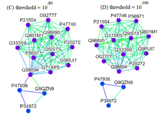 |
Fig. 6 Thresholded sequence similarity network graphs of the Cannabinoid Receptor family with the threshold distance of 10–20 (A), 10–50 (B), 10–80 (C), and 10–100 (D). Nodes and edges are respectively colored by the value of their closeness centrality and betweenness centrality according to the color bar.
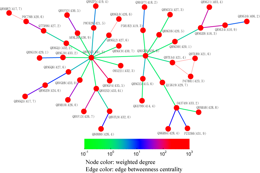
Fig. 7 A partial minimum spanning tree of Olfactory Receptors near the hub sequence Q8VFK7. Nodes are colored based on their closeness centrality values which are labeled in the parentheses. Edges are colored based on their betweenness centrality values. Thin edges represent those sequence pairs of zero distance.
(II) In the bottom-up navigation, the database containing the base dataset of 2841 GPCRs is selected, and the query sequence is uploaded or entered at the homepage in the FASTA format. SeQuery determines if it is a GPCR based on its distance to the sequences in the base dataset. If so, as shown in Figure 5, SeQuery will display the graph of network connections between the query sequence and its neighbors at the first level of clustering, as well as information related to the overall cluster and its closest neighbor. The role of this cluster in the GPCR network can be further investigated at the second or third level of clustering.
Centrality measures for the sequence similarity network of GPCRs
In a network, central nodes are those in the thick of things. To evaluate the centrality of important nodes, we consider four different centrality measures, namely the weighted degree, closeness, betweenness, and eigenvector centralities (as defined in Figure 8), for an all-to-all, undirected, and weighted graph G := (V, E) with |V| nodes and |E| edges. The weight matrix W of the graph has weights wuv for the edges connecting nodes u and v (∀u,v∈V). Equivalently, we define a distance matrix D with elements duv, where duv ≡ wuv–1–1.
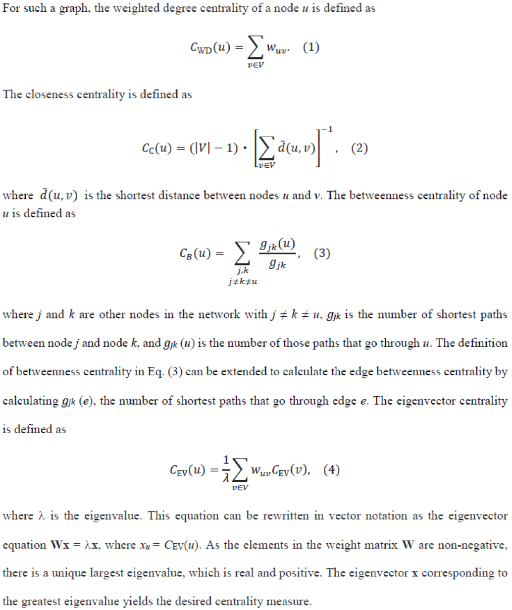
Fig. 8 Definition of various centrality measures, including weighted degree, closeness, betweenness, and eigenvector centralities.
In applying graph theory to study the sequence similarity network of GPCRs, we use these centrality indices to characterize important nodes or edges within the network. The weighted degree centrality of a sequence (or a node) is used to characterize its overall connectivity to other sequences in the network. The closeness centrality of a sequence measures the reciprocal of the sum of the length of the shortest paths between the sequence and all other sequences; the more central a sequence is, the closer it is to all other sequences. In graph theory, the betweenness centrality of a node/edge is the number of the shortest paths that pass through the node/edge; a node/edge with higher betweenness centrality would have more control over the network. Lastly, the eigenvector centrality measures the influence of a node in a network; a high eigenvector score means that a node is connected to many nodes of high scores. In general, the closeness/weighted degree/eigenvector centrality measures have similar patterns in a complex network; while the betweenness centrality is characteristically different from the other three measures and has a dynamic role in representing the information flow of the network (31). For the study of GPCRs, the first three centrality measures can be used to find the most representative/influential sequence of a GPCR cluster, sub-family, or family. The betweenness centrality can be used to find particular sequences (nodes) or sequence pairs (edges) that bridge different domains in the sequence space of GPCRs; these sequences or sequence pairs could play a key role in the evolution of GPCRs.